
![]()

In case you wonder about the name and what cowplot package can do for you, check out the introduction from cowplot’s github page.
The cowplot package provides various features that help with creating publication-quality figures, such as a set of themes, functions to align plots and arrange them into complex compound figures, and functions that make it easy to annotate plots and or mix plots with images. The package was originally written for internal use in the Wilke lab, hence the name (Claus O. Wilke’s plot package). It has also been used extensively in the book Fundamentals of Data Visualization.
One can install cowplot packge from CRAN with
install.packages("cowplot")
Let us load the cowplot package and check its version.
library(cowplot)
packageVersion("cowplot")
1.1.1’
We will also be loading tidyverse for using ggplot2 and palmerpenguins package for palmer penguins data.
library(tidyverse)
library(palmerpenguins)
theme_set(theme_bw(base_size=16))
To illustrate the use cowplot to combine multiple plots made with ggplot2 in R, we will create two plots using penguins data.
At first, we make a scatterplot using geom_point() in ggplot2 and save the plot object in a variable.
p1 <- penguins %>%
  ggplot(aes(x=bill_depth_mm,body_mass_g, color=species))+
  geom_point()
p1
Similarly, we make another plot, this time a density plot using penguins data and save it as a variable
p2 <- penguins %>%
  drop_na()%>%
  ggplot(aes(x=body_mass_g, fill=species))+
  geom_density(alpha=0.5)
p2
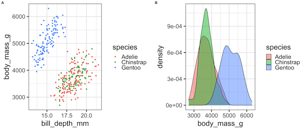
How to combine two plots side by side with cowplot’s plot_grid()?
We now have the two plots made with ggplot2 ready and we would like to combine the two plots into a single plot using cowplot. The main function to combine plots with cowplot is plot_grid() function.
Here we provide two plots as argument and specify labels and label sizes.
plot_grid(p1,
          p2,
          labels = c('A', 'B'),
          label_size = 12)

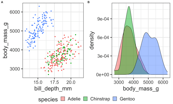
How to combine two plots side by side with shared legend using cowplot?
Our first attempt to combine two plots with cowplot was successful. However, you can see that both the plots have the same legends repeated twice. It would be better to remove the redundancy by having a shared legend. In this example below we will see how to have a common legend for our plot combined with cowplot.
We will use plot_grid() function with no legend for each plot we have and store the result as a variable.
combined_plot <- plot_grid(p1 + theme(legend.position = "none"),
          p2 + theme(legend.position = "none"),
          labels = c('A', 'B'), label_size = 12)
Next, we will create a new variable with legend from one of the plots such that the legend is at the bottom of our new combined plot.
legend <- get_legend(
  # create some space to the left of the legend
  p2 +
    guides(color = guide_legend(nrow = 1)) +
    theme(legend.position = "bottom")
)
We can combine the two new plot objects with plot_grid() function in cowplot. Note that in addition to the plot objects we also specify relative heights (using “rel_heights”) for these two plot objects to get a combined plot with shared legend at the bottom.
plot_row <- plot_grid(combined_plot,
                      legend,
                      ncol = 1,
                      rel_heights = c(1, .1))
ggsave("join_ggplots_with_shared_legend_cowplot.png", width=10,height=6)

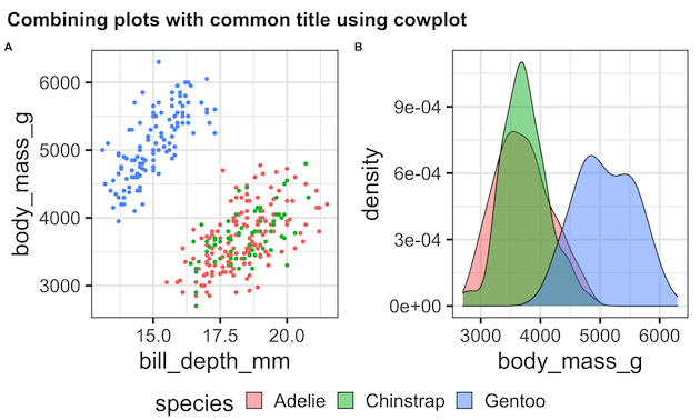
How to combine two plots with shared title using cowplot?
Now let us see how can we have common title for our combined plot with cowplot. To create a common title we will use draw_label() function in cowplot and use ggdraw() to have a common title.
# now add the title
title <- ggdraw() +
  draw_label(
    "Combining plots with common title using cowplot",
    fontface = 'bold',
    x = 0,
    hjust = 0,
    size = 24,
  ) +
  theme(
    # add margin on the left of the drawing canvas,
    # so title is aligned with left edge of first plot
    plot.margin = margin(0, 0, 0, 7)
  )
Now we can combine the title object with the main object to get a plot with shared title.
plot_grid(
  title,
  plot_row,
  ncol = 1,
  # rel_heights values control vertical title margins
  rel_heights = c(0.1, 1)
)
ggsave("join_ggplots_with_shared_legend_and_title_cowplot.png", width=10,height=6)
Explore the Complete ggplot2 Guide
35+ tutorials with code: scatterplots, boxplots, themes, annotations, facets, and more—tested and beginner-friendly.
Visit the ggplot2 Hub → No fluff—just code and visuals.


