How to make Annotated heatmap with Seaborn in Python

In this tutorial, you’ll learn how to create an annotated heatmap in Python using Seaborn, a powerful data visualization library built on Matplotlib. We’ll start by generating a basic heatmap with the heatmap() function to visualize data in a color-coded grid. Then, we’ll take it a step further by adding annotations—first as plain text values inside each cell, and then with percentage symbols for a more informative and presentation-ready look.

👉 Want more? Explore the full Seaborn Tutorial Hub with 35+ examples, code recipes, and best practices.

Along the way, you’ll see how to control text formatting, adjust font styles, and ensure annotations are clear and readable. By the end, you’ll be able to build Seaborn annotated heatmaps that make patterns in your data instantly understandable—perfect for reports, dashboards, and data analysis workflows.

Let us load the packages needed.

import seaborn as sns
import pandas as pd
import matplotlib.pyplot as plt
import numpy as np

We will use the S&P index’s monthly returns data from year 2000 to make a heatmap. We will load the data directly from the web. And the data looks like this.

sp500_long = pd.read_csv("SP500_monthly_returns.tsv", sep="\t")
sp500_long.head()

          date. 	returns	      month	year
0	2000-01-31	-0.041753	January	2000
1	2000-02-29	-0.020108	February	2000
2	2000-03-31	0.096720	March	2000
3	2000-04-28	-0.030796	April	2000
4	2000-05-31	-0.021915	May	2000

Let us reshape the data to a matrix form with months on rows and year as columns using Pandas’ pivot() function. And also convert the returns to percentage by multiplying by 100.

sp500 = (
    sp500_long
    .pivot(index="month", columns="year", values="returns")
)
sp500 = sp500*100

Heatmap with Seaborn

Let us make a simple heatmap with the data.

f, ax = plt.subplots(figsize=(6, 9))
sns.heatmap(sp500, 
            fmt="",
            cmap="Spectral",
            linewidths=.5, 
            ax=ax)
plt.yticks(rotation=0)
plt.xticks(rotation=45)
plt.title("S&P 500 Monthly Returns as Heatmap",size=20)
plt.savefig('Seaborn_heatmap.png')

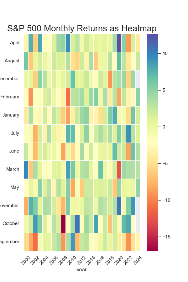
Our first attempt at heatmap with Seaborn has got the order of months on rows wrong. Let us fix the order of months using Pandas Categorical function and sorting in the right order. We also transpose the data so as to years are in the rows and months are in columns.

# Convert the index (months) to a Categorical type with the correct order
month_order = ['January', 'February', 'March', 'April', 'May', 'June', 
               'July', 'August', 'September', 'October', 'November', 'December']

sp500.index = pd.Categorical(sp500.index, categories=month_order, ordered=True)
sp500 = sp500.sort_index()  # Sort to ensure the order is applied corr
sp500=sp500.transpose()

Heatmap with Seaborn’s heatmap() function

Let us try again to make the heatmap with Seaborn.

f, ax = plt.subplots(figsize=(6, 9))
sns.heatmap(sp500, 
            #annot=sp500.map(format_percentage), 
            fmt="",
            cmap="Spectral",
            linewidths=.5, 
            ax=ax)
plt.yticks(rotation=0)
plt.xticks(rotation=45)
plt.title("S&P 500 Monthly Returns as Heatmap",size=20)
plt.savefig('sp500_returns_heatmap.png')

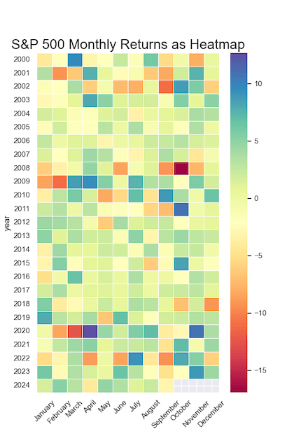
Now the months are in right order as we wanted.

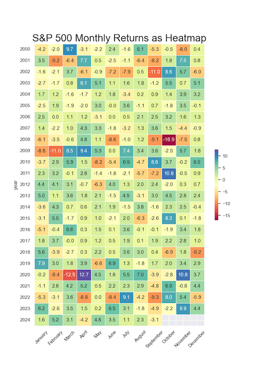
Add annotation to Heatmap with Seaborn’s heatmap() function

We can add annotations to a heatmap using the annot argument. In the example below, we format the values with a custom function to display the return values directly on the heatmap.

# Function to round
def roundit(value):
    return f'{value:.1f}'

We use annot argument with the data in the right format using map() function to format each element of our data.

f, ax = plt.subplots(figsize=(9, 12))
sns.heatmap(sp500, 
            annot=sp500.map(roundit), 
            fmt="",
            cmap="Spectral",
            linewidths=.5, 
            ax=ax,
            cbar_kws={"shrink": 0.25})
plt.yticks(rotation=0)
plt.xticks(rotation=45)
plt.title("S&P 500 Monthly Returns as Heatmap",size=24)
plt.savefig('sp500_returns_as_annotated_heatmap.png')

Add annotation with percent symbol to Heatmap with Seaborn’s heatmap() function

We can also add a percent symbol to the annotations using a similar approach as above. This is done by setting the annot argument in the heatmap() function and applying a custom formatting function to display each value with a percentage sign.

# Function to format annotation as percentage
def format_percentage(value):
    return f'{value:.1f}%'

f, ax = plt.subplots(figsize=(9, 12))
sns.heatmap(sp500, 
            annot=sp500.map(format_percentage), 
            fmt="",
            cmap="Spectral",
            linewidths=.5, 
            ax=ax,
            cbar_kws={"shrink": 0.25})
plt.yticks(rotation=0)
plt.xticks(rotation=45)
plt.title("S&P 500 Monthly Returns as Heatmap",size=24)
plt.savefig('sp500_returns_as_annotated_heatmap_with_percent_symbol.png')