In this post, we will learn how to combine two plots side-by-side using four different approaches. First, we will show how we can use facet_wrap() function in ggplot2, if we are interested in similar plots (small multiples) side by side. Next three approaches are more general, i.e. combining any two plots side by side using the R packages patchwork, cowplot, and gridExtra.
Let us get started by loading all the libraries needed.
library(palmerpenguins)
library(tidyverse)
library(cowplot)
library(gridExtra)
library(patchwork)
theme_set(theme_bw(16))
We will use palmer penguins data to make plots and arrange them side by side.
penguins |>
  head()

# A tibble: 6 × 8
  species island    bill_length_mm bill_depth_mm flipper_length_mm body_mass_g
  <fct>   <fct>              <dbl>         <dbl>             <int>       <int>
1 Adelie  Torgersen           39.1          18.7               181        3750
2 Adelie  Torgersen           39.5          17.4               186        3800
3 Adelie  Torgersen           40.3          18                 195        3250
4 Adelie  Torgersen           NA            NA                  NA          NA
5 Adelie  Torgersen           36.7          19.3               193        3450
6 Adelie  Torgersen           39.3          20.6               190        3650
# ℹ 2 more variables: sex <fct>, year <int>
side by side with facet_wrap() (small multiples)
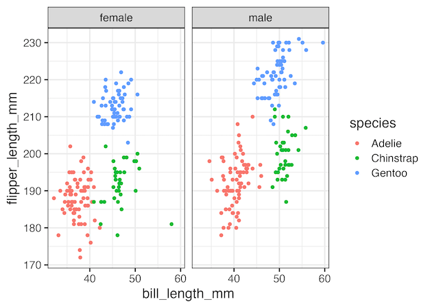
When the two or more plots that we want to arrange side by side is of small multiples, we can use facet_wrap() function to arrange them side by side.
penguins |>
  drop_na() |>
  ggplot(aes(x=bill_length_mm, y=flipper_length_mm, color=species))+
  geom_point()+
  facet_wrap(~sex)
ggsave("side_by_side_smal_multiples_plot_ggplot2_facet_wrap.png")

Let us consider an example, where we have two different types of plots. One is a scatter plot as given below.
p1 <- penguins |>
  drop_na() |>
  ggplot(aes(bill_length_mm,bill_depth_mm, color=species))+
  geom_point()
print(p1)
ggsave("how_to_combine_plots_side_by_side_p1.png")

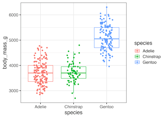
And the other is a boxplot as given below.
p2 <- penguins |>
  drop_na() |>
  ggplot(aes(x=species, y= body_mass_g, color=species))+
  geom_boxplot(outlier.shape = NA)+
  geom_jitter(width=0.2)
p2
ggsave("how_to_combine_plots_side_by_side_p2.png")
We have saved both the plots into two variables, so that it can be reused later.
Side by Side plots with patchwork
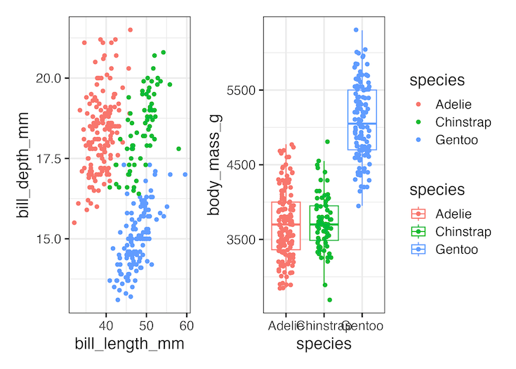
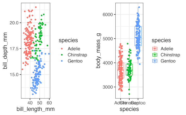
One of the ways to combine two plots side by side is to use the R package patchwork’s + function.
p1 +p2
ggsave("side_by_side_plots_ggplot2_patchwork.png")

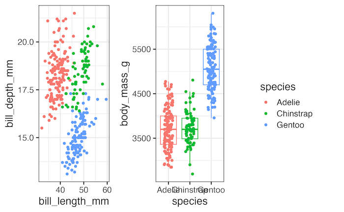
And here is how it looks after arranging them side by side. We can make it better by collecting the legends of the plot and putting them in a common area. We can collect the legends using plot_layout() function as show below.

p1 +p2 + plot_layout(guides = 'collect')
ggsave("side_by_side_plots_common_legends_ggplot2_patchwork.png")

Side by Side plots with cowplot
We can use plot_grid() function in cowplot package to combine two plots side by side.
plot_grid(p1, p2)
ggsave("side_by_side_plots_ggplot2_cowplot_plot_grid.png")


legend <- get_legend( p1 )
# Combine plot and legend using plot_grid()
plot_grid(p1+theme(legend.position="none"),
          p2 +theme(legend.position="none"),
          legend,
          ncol=3)
ggsave("side_by_side_plots_common_legend_ggplot2_cowplot_plot_grid.png")
Side by Side plots with gridExtra
We can also use gridExtra package to arrange plots side by side using grid.arrange() function.
gridExtra::grid.arrange(p1, p2, ncol = 2)

ggsave("side_by_side_plots_ggplot2_gridExtra.png")
And here is how we can use the grabbed legend shown before to combine the legends in one place with grid.arrange() function in gridExtra.
gridExtra::grid.arrange( p1+theme(legend.position = "none"),
                         p2+theme(legend.position = "none"),
                         legend, ncol = 3)
With gridExtra, to save the plot as png file, we have grab the ggplot2 object and pass it to ggsave as shown below.

gridExtra::grid.arrange( p1+theme(legend.position = "none"),
                         p2+theme(legend.position = "none"),
                         legend1, ncol = 3)

# Create a grob from the arranged plots
grob <- arrangeGrob( p1+theme(legend.position = "none"),
                         p2+theme(legend.position = "none"),
                         legend1, ncol = 3)

# Use ggsave to save the grob
ggsave("side_by_side_with_common_legend_ggplot2_gridExtra.png", grob)
Explore the Complete ggplot2 Guide
35+ tutorials with code: scatterplots, boxplots, themes, annotations, facets, and more—tested and beginner-friendly.
Visit the ggplot2 Hub → No fluff—just code and visuals.