
In this tutorial, we will learn how to make raincloud plots with the R package ggdist. In an earlier post, we learned how to make rain cloud plots with half violinplot, kind of from scratch. However, ggdist, an R package “that provides a flexible set of ggplot2 geoms and stats designed especially for visualizing distributions and uncertainty”, makes it easy to create rain cloud plots using special geoms.
We can use ggdist’s geom_dotsinterval() / stat_dotsinterval() functions to make rain cloud plots, which is a combination of half-eyes or half violin plot, boxplot and beeswarm/dotplots.
Let us load the packages needed to make rain cloud plot.
library(tidyverse)
library(palmerpenguins)
library(ggdist)
theme_set(theme_bw(16)
packageVersion("ggdist")
## [1] '3.2.0'
Half eye or Half Violin Plot with ggdist
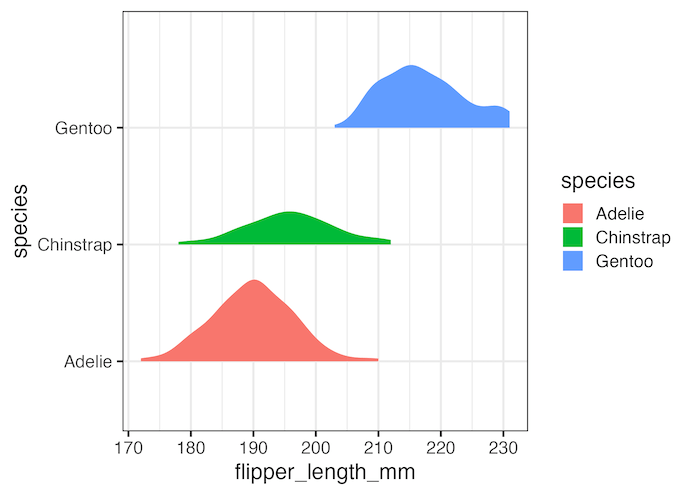
We will build rain cloud plot step by step using ggdist’s function. First, let us make density/ridge/half-eye/half-violin plot. With ggdist, we can make half violin plot (or half eye) using stat_slab() function.
penguins %>%
  ggplot(aes(x=flipper_length_mm, y=species, fill=species))+
  stat_slab(aes(thickness = stat(pdf*n)),
                scale = 0.7)
ggsave("ggdist_raincloud_plot.png")
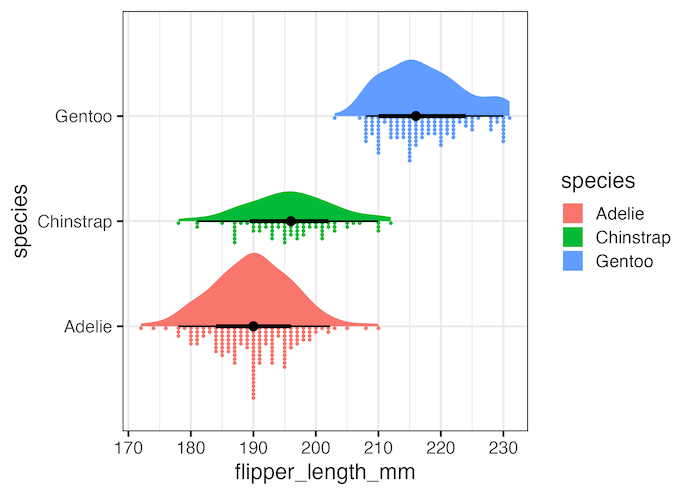
Simple rain cloud plot with ggdist
By adding “stat_dotsinterval” function we can make rain cloud plot. Here with “side=bottom” argument makes the dot plots to be at the bottom of the density plot to make it look like rain cloud plot.
penguins %>%
  ggplot(aes(x=flipper_length_mm, y=species, fill=species))+
  stat_slab(aes(thickness = stat(pdf*n)),
                scale = 0.7) +
  stat_dotsinterval(side = "bottom",
                    scale = 0.7,
                    slab_size = NA)
ggsave("ggdist_raincloud_plot_with_summary_interval.png")
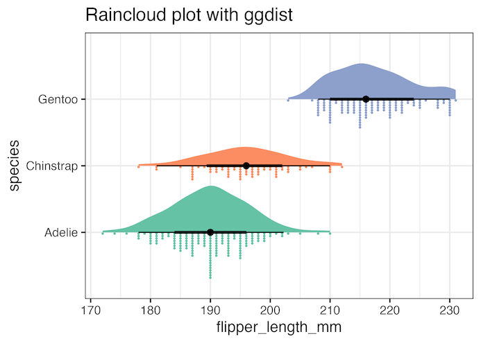
Simple customizations to rain cloud plot
The above rain cloud plot is default one. We can improve the plot simply changing the color palette used and removing the legend as it is redundant. And also add a title to the rain cloud plot
penguins %>%
  ggplot(aes(x=flipper_length_mm, y=species, fill=species))+
  stat_slab(aes(thickness = stat(pdf*n)),
                scale = 0.7) +
  stat_dotsinterval(side = "bottom",
                    scale = 0.7,
                    slab_size = NA) +
  scale_fill_brewer(palette = "Set2") +
  theme(legend.position = "none")+
  labs(title="Raincloud plot with ggdist")
ggsave("ggdist_raincloud_plot_with_datapoints_as_drops.png")
Explore the Complete ggplot2 Guide
35+ tutorials with code: scatterplots, boxplots, themes, annotations, facets, and more—tested and beginner-friendly.
Visit the ggplot2 Hub → No fluff—just code and visuals.


