Last updated on August 29, 2025

In this tutorial, you’ll learn 9 tips to make your Seaborn scatter plots publication-ready. We’ll use the popular Palmer Penguins dataset to explore culmen length, flipper length, body mass, and species differences.
👉 Want more? Explore the full Seaborn Tutorial Hub with 35+ examples, code recipes, and best practices.
With Seaborn in Python, we can make scatter plots in multiple ways, like lmplot(), regplot(), and scatterplot() functions.
We will use Seaborn’s scatterplot() function to make scatter plots in Python. One of the benefits of using scatterplot() function is that one can easily overlay three additional variables on the scatterplot by modifying color with “hue”, size with “size”, and shape with “style” arguments.
Let us load the packages we need.
import matplotlib.pyplot as plt
import pandas as pd
import seaborn as sns

Penguin Data were collected and made available by Dr. Kristen Gorman and the Palmer Station, Antarctica LTER.
And Thanks to Alison Horst for making the data easily available.
We will load the simplified data directly from github page.
penguins_data="https://raw.githubusercontent.com/datavizpyr/data/master/palmer_penguin_species.tsv"
penguins_df = pd.read_csv(penguins_data, sep="\t")
We can see that we four numerical variables corresponding to three Penguin species. Check the github page for nice illustrations of the body measurements.
penguins_df.head()
species	island	culmen_length_mm	culmen_depth_mm	flipper_length_mm	body_mass_g	sex
0	Adelie	Torgersen	39.1	18.7	181.0	3750.0	MALE
1	Adelie	Torgersen	39.5	17.4	186.0	3800.0	FEMALE
2	Adelie	Torgersen	40.3	18.0	195.0	3250.0	FEMALE
3	Adelie	Torgersen	NaN	NaN	NaN	NaN	NaN
4	Adelie	Torgersen	36.7	19.3	193.0	3450.0	FEMALE
Let us get started. In this tutorial, we will learn 9 tips to make publication quality scatter plot with Python. We will start with how to make a simple scatter plot using Seaborn’s scatterplot() function. And then we will use the features of scatterplot() function and improve and make the scatter plot better in multiple steps.
1. How To Make Simple Scatter Plot with Seaborn’s scatterplot()?
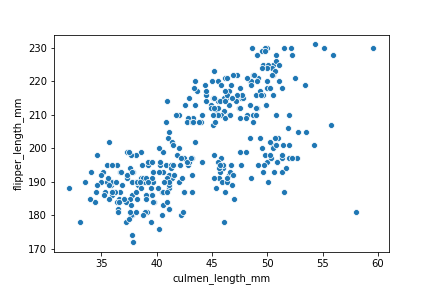
Let us get started making scatter plots with Penguin data using Seaborn’s scatterplot() function. First, we will make a simple scatter plot between two numerical variables from the dataset, culmen_length_mm and filpper_length_mm.
We can use Seaborn’s scatterplot() specifying the x and y-axis variables with the data as shown below.
sns.scatterplot(x="culmen_length_mm",
                y="flipper_length_mm",
                data=penguins_df)
And we get a simple scatter plot like this below.
2. How To Increase Figure Size in Python?
By default, Seaborn creates relatively small plots. For clarity in reports or presentations, you can increase the figure size with Matplotlib’s figure() function.
# specify figure size with Matplotlib
plt.figure(figsize=(10,8))
sns.scatterplot(x="culmen_length_mm",
                y="flipper_length_mm",
                data=penguins_df)
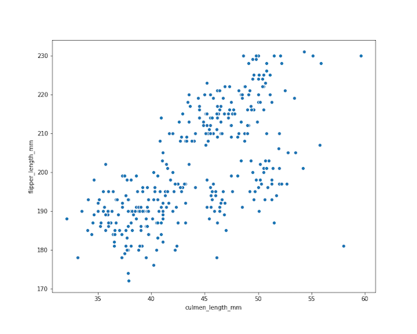
In the example here, we have specified the figure size with figsize=(10,8). Now the scatter plot is larger and easier to interpret.
3. How To Increase Axes Tick Labels in Seaborn?
Bigger plots also need readable axis labels. Use Seaborn’s plotting_context() to scale font sizes for tick labels. We can increase Axes tick labels using Seaborn’s plotting_context() function. In this example, we use plotting_context() function with the arguments ‘”notebook”,font_scale=1.5’.
# specify figure size with Matplotlib
plt.figure(figsize=(10,8))
# Increase axis tick label with plotting_context in Seaborn
with sns.plotting_context("notebook",font_scale=1.5):
    sns.scatterplot(x="culmen_length_mm",
                y="flipper_length_mm",
                data=penguins_df)
Now we have a better looking scatter plot between Penguin’s Culmen length and Flipper Length with easily readable axis tick labels.

4. How To Change Marker Size in Seaborn Scatterplot?
Sometimes the default marker size is too small, making points hard to see. You can use the s parameter in Seaborn’s scatterplot() to adjust marker size.
# Set common  plotting_context for all the plots
# in the script/notebook
sns.set_context("notebook", font_scale=1.5)
# set figure size
plt.figure(figsize=(10,8))
# change marker size with s=100 in
# Seaborn scatterplot()
sns.scatterplot(x="culmen_length_mm",
                    y="flipper_length_mm",
                    s=100,
                    data=penguins_df)
plt.savefig("How_To_Change_Marker_Size_Seaborn_ScatterPlot.png",
                    format='png')
The scatter plot now has larger, clearer points, making it easier to interpret individual observations.

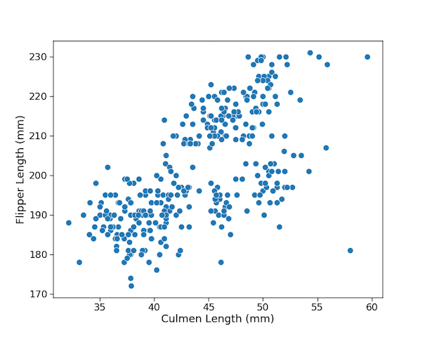
5. How To Change Axis Labels and Size with Matplotlib for Seaborn Scatterplot?
Notice that, our x and y axis labels are the same names as in Penguin’s data frame. By default, Seaborn uses variable names from the dataset as axis labels. You can make your chart more presentation-friendly by customizing labels with Matplotlib’s xlabel() and ylabel().
We use Matplotlibs’ xlabel() and ylabel() functions to change the labels and increase their font sizes.
plt.figure(figsize=(10,8))
sns.scatterplot(x="culmen_length_mm",
                    y="flipper_length_mm",
                    s=100,
                    data=penguins_df)
# set x-label
plt.xlabel("Culmen Length (mm)", size=24)
plt.ylabel("Flipper Length (mm)", size=24)
plt.savefig("Customize_Axis_Labels_Scatter_Plot_Penguins_data_Seaborn.png",
                    format='png')
We have customized the x-axis and y-axis labels and also increased label’s font sizes.
6. How To Color Scatter Plot by a Variable with Seaborn’s scatterplot()?
Adding a third variable as color is easy in Seaborn with the hue argument. Let’s color points by penguin species. In this example, we have colored the data points by the “species” variable using hue="species".
plt.figure(figsize=(10,8))
sns.scatterplot(x="culmen_length_mm",
                y="flipper_length_mm",
                s=100,
                hue="species",
                data=penguins_df)
plt.xlabel("Culmen Length (mm)")
plt.ylabel("Flipper Length (mm)")
plt.savefig("Color_scatterplot_by_variable_with_hue_Seaborn_scatterplot.png",
                    format='png',dpi=150)
By coloring data points by a variable in the scatter plot, we have added third variable to the plot. Seaborn automatically represents the third variable with the legend describing colors to the plot.

7. How To Change Shape by a Variable in Scatter Plot with Seaborn’s scatterplot()?
You can represent another categorical variable using the style argument. For example, use penguin sex to change marker shapes.
plt.figure(figsize=(10,8))
sns.scatterplot(x="culmen_length_mm",
                y="flipper_length_mm",
                s=100,
                style="sex",
                data=penguins_df)
plt.xlabel("Culmen Length (mm)")
plt.ylabel("Flipper Length (mm)")
plt.savefig("Add_shape_scatterplot_by_variable_with_hue_Seaborn_scatterplot.png",
                    format='png',dpi=150)
Now male and female penguins have different marker shapes, adding another layer of information.

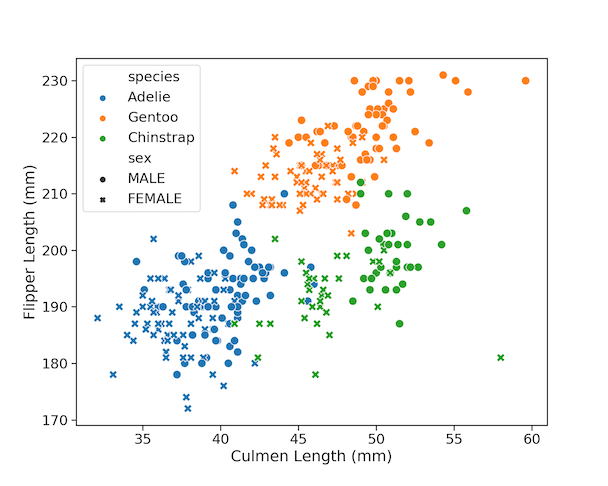
8. How To Change Color and Shape in Scatter Plot by Two Variables in Seaborn’s scatterplot()?
One of the advantages of Seaborn’s scatterplot function is that we can easily combine hue and style to color data points by one variable and change marker’s shape based on another variable. This way we are displaying four variables in a single scatter plot.
plt.figure(figsize=(10,8))
sns.scatterplot(x="culmen_length_mm",
                y="flipper_length_mm",
                s=100,
                hue="species",
                style="sex",
                data=penguins_df)
plt.xlabel("Culmen Length (mm)")
plt.ylabel("Flipper Length (mm)")
plt.savefig("Color_and_shape_by_variable_Seaborn_scatterplot.png",
                    format='png',dpi=150)
We have colored data points by Penguin species and changed marker shapes by penguin’s sex. This enables us to visualize the relationship between culmen length and flipper length with respect to species and sex.
9. How to Change Color, Shape and Size By Three Variables in Seaborn’s scatterplot()
Finally, Seaborn’s scatterplot() can also map a third categorical/continuous variable to point size, creating a bubble plot.
plt.figure(figsize=(12,10))
sns.scatterplot(x="culmen_length_mm",
                y="flipper_length_mm",
                size="body_mass_g",
                hue="species",
                style="sex",
                data=penguins_df)
plt.xlabel("Culmen Length (mm)")
plt.ylabel("Flipper Length (mm)")
plt.savefig("Change_Size_Color_Shape_by_three_variables_Seaborn_scatterplot.png",
                    format='png',dpi=150)
In this tutorial, we started with a basic Seaborn scatter plot and progressively improved it with:
• Larger figure sizes and readable axis labels
• Bigger markers and customized labels
• Added variables with color, shape, and size
These tips will help you make publication-quality scatter plots for presentations, papers, or data storytelling.

Although the ability to add three variables is nice, it can also affect the easy interpretability of the plots. There are better ways to show multiple variables.
Frequently Asked Questions (FAQs)
What is the difference between Seaborn scatterplot() and Matplotlib plt.scatter()?
Seaborn scatterplot() adds built-in support for mapping additional variables (color, size, shape) and integrates with pandas DataFrames, while plt.scatter() is lower-level and requires more manual setup.
Can I add a regression line to Seaborn scatter plots?
Yes. Instead of scatterplot(), you can use Seaborn’s regplot() or lmplot(), which draw regression lines along with scatter points automatically.
How do I handle missing values when plotting with Seaborn?
You should drop rows with NaN in the x or y columns before plotting. For example: df.dropna(subset=["culmen_length_mm","flipper_length_mm"]).
How can I save a Seaborn scatter plot with high resolution?
Use Matplotlib’s savefig() with the dpi parameter, e.g. plt.savefig("scatter.png", dpi=300) to create a high-resolution image for publications.
Is Seaborn scatterplot() suitable for very large datasets?
Scatterplots can become slow and cluttered with millions of points. For large datasets, consider downsampling, using alpha for transparency, or trying Seaborn’s kdeplot() or hexbin plots in Matplotlib.
What are the challenges of adding three or more variables to a scatter plot?
Encoding color, shape, and size at the same time can make scatter plots cluttered and hard to interpret. Better alternatives include:
- Faceting with Seaborn’s FacetGrid – split plots into panels by category instead of mixing too many shapes/colors.
- Pair plots (sns.pairplot) – show many numeric variables in a grid of scatter plots.
- Dimensionality reduction (PCA, t-SNE) – reduce many features to 2D for plotting.
- Interactive plots (Plotly/Altair) – add hover tooltips instead of encoding every variable visually.