How to Order Months Chronologically in ggplot2 (Fixing Alphabetical Sort)

Last updated on November 24, 2025

One of the most common frustrations for R beginners is plotting time-series data. You create a beautiful bar chart, but ggplot2 places April before January.

Why does this happen? By default, R treats text variables (character strings) alphabetically. Since “A” comes before “J”, April appears first.

In this tutorial, we will learn how to force R to respect chronological order by converting our data into Factors.

library(tidyverse)
theme_set(theme_bw(16))

1. Creating the Example Data

Let’s generate a sample dataset containing monthly stock returns. We will use month.abb (a built-in R vector containing “Jan”, “Feb”, etc.) to create our month column.

Note: The months variable here is stored as a Character (text) string.

year <- c("2024")
set.seed(12345)
df <- expand_grid(year, months=month.abb) |>
  mutate(returns= rnorm(n=12,mean=15,sd=20)) |>
  mutate(up_down=ifelse(returns>0, "+ve", "-ve"))

df

# A tibble: 12 × 4
   year  months returns up_down
   <chr> <chr>    <dbl> <chr>  
 1 2024  Jan      26.7  +ve    
 2 2024  Feb      29.2  +ve    
 3 2024  Mar      12.8  +ve    
 4 2024  Apr       5.93 +ve    
 5 2024  May      27.1  +ve    
 6 2024  Jun     -21.4  -ve    
 7 2024  Jul      27.6  +ve    
 8 2024  Aug       9.48 +ve    
 9 2024  Sep       9.32 +ve    
10 2024  Oct      -3.39 -ve    
11 2024  Nov      12.7  +ve    
12 2024  Dec      51.3  +ve

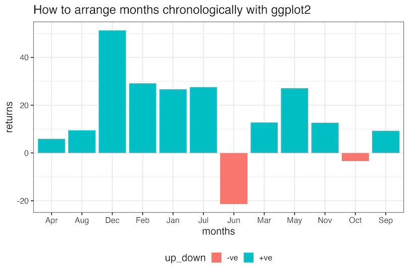
2. The Problem: The Default Alphabetical Plot

If we plot this data immediately, ggplot2 sees the months column as simple text. It sorts the X-axis alphabetically: Apr, Aug, Dec, Feb…

When we make a barplot with months on x-axis and returns on y-axis, we get a barplot with months on x-axis ordered alphabetically.

df |>
  ggplot(aes(x=months, y=returns, fill=up_down))+
  geom_col()+
  theme(legend.position="bottom")+
  labs(title="How to arrange months chronologically with ggplot2")
ggsave("How_to_arrange_months_in_right_order_ggplot2.png", width=9, height=6)

This makes the data nearly impossible to interpret as a time series

How to arrange months in right order with ggplot2

The Solution: Using Factors to Fix the Order

To fix this, we need to tell R that months is not just text, but a categorical variable with a specific order. We do this by converting it to a Factor.

We use the levels argument to define the correct order. R provides a convenient built-in constant month.abb which lists months from Jan to Dec.

If you have abbreviations (Jan, Feb): Use levels = month.abb

If you have full names (January, February): Use levels = month.name

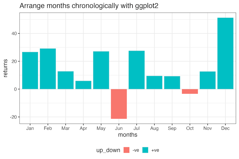
To reorder months in the right order, i.e. chronologically, we first convert the month variable as factor with levels in the right chronological order. Then we can make the barplot as before.


# Convert 'months' to a factor with specific levels
df_fixed <- df |>
  mutate(months = factor(months, levels = month.abb))

df_fixed |>
  ggplot(aes(x=months, y=returns, fill=up_down))+
  geom_col()+
  theme(legend.position="bottom")+
  labs(title="Arrange months chronologically with ggplot2")
ggsave("arrange_months_in_right_order_ggplot2.png", width=9, height=6)

By explicitly defining the levels, ggplot2 now understands the hierarchy of the data and plots January through December in the correct chronological order. And we get the months ordered correctly as we wanted.

Arranging months in right order with ggplot2

3. Plotting in Reverse Chronological Order

Sometimes you want to show the most recent data first (e.g., December at the top or left). To do this, we simply reverse the list of levels using the rev() function.

# Reverse the order of levels
df |>
  mutate(months = factor(months, levels = rev(month.abb))) |>
  ggplot(aes(x = months, y = returns, fill = up_down)) +
  geom_col() +
  labs(title = "Reverse Chronological Order (Dec to Jan)")

Handling Date Objects (The Automated Way)

In real-world settings, you rarely type out “Jan”, “Feb” manually. You usually start with a proper Date column (e.g., 2024-01-01).

We can use the lubridate package to extract the month name and set the order automatically. This is much faster and less prone to typing errors.

Let’s create a dataset with a standard Date column:

library(tidyverse)
theme_set(theme_bw())

# Create a sequence of Dates
df_dates <- tibble(
  date_col = seq(as.Date("2024-01-01"), as.Date("2024-12-01"), by = "month"),
  returns = rnorm(12, mean=10, sd=15)
) |> 
  mutate(up_down = ifelse(returns > 0, "+ve", "-ve"))

df_dates |>
  head()

date_col returns up_down
2024-01-01	-15.219732	-ve		
2024-02-01	1.910872	+ve		
2024-03-01	22.890982	+ve		
2024-04-01	18.568514	+ve		
2024-05-01	-7.167192	-ve		
2024-06-01	4.887988	+ve

df_dates |>
  # label=TRUE creates an Ordered Factor automatically
  mutate(month_name = month(date_col, label = TRUE, abbr = TRUE)) |>
  ggplot(aes(x = month_name, y = returns, fill = up_down)) +
  geom_col() +
  labs(title = "Automatic Ordering with Lubridate")
ggsave("ordering_date_objects_with_lubridate_ggplot2.png")

This is better, because when you use label = TRUE, R internally creates an Ordered Factor. You don’t need to manually type out levels = c(“Jan”, “Feb”…).