Correlation Heatmap wiht Corrr

In this post, we will learn how to make a simle correlation heatmap of numerical variables in a dataframe using Corrr R package. The R package Corrr starting from version 0.4.4 has a autoplot() function enables you to make simple correllation heatmap in addition to correlation dotplot and network plot. Thanks to Emil Hvitfeldt’s tweet announcing the new release of corr.

Let us get started by loading the packages and checking the version of corrr package.

library(tidyverse)
library(palmerpenguins)
library(corrr)
packageVersion("corrr")

## [1] '0.4.4'

We will work with dataframe containing only the numerical variables.

penguins <- penguins %>%
  drop_na() %>%
  select(-year) %>%
  select(where(is.numeric))

penguins  %>% head()

## # A tibble: 6 × 4
##   bill_length_mm bill_depth_mm flipper_length_mm body_mass_g
##            <dbl>         <dbl>             <int>       <int>
## 1           39.1          18.7               181        3750
## 2           39.5          17.4               186        3800
## 3           40.3          18                 195        3250
## 4           36.7          19.3               193        3450
## 5           39.3          20.6               190        3650
## 6           38.9          17.8               181        3625

As we in the previous post, we can compute correlation of all numerical variables against all other variables using corrr’s correlate() function by using input data as a dataframe.
We get a symmetric tibble with all correlation computed by Pearson correlation method.

penguins %>% 
  correlate()

## Correlation computed with
## • Method: 'pearson'
## • Missing treated using: 'pairwise.complete.obs'

## # A tibble: 4 × 5
##   term              bill_length_mm bill_depth_mm flipper_length_mm body_mass_g
##   <chr>                      <dbl>         <dbl>             <dbl>       <dbl>
## 1 bill_length_mm            NA            -0.229             0.653       0.589
## 2 bill_depth_mm             -0.229        NA                -0.578      -0.472
## 3 flipper_length_mm          0.653        -0.578            NA           0.873
## 4 body_mass_g                0.589        -0.472             0.873      NA

Correlation heatmap with autoplot()

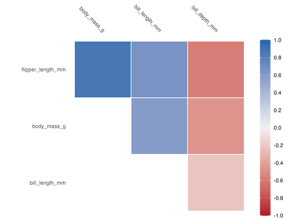
To make a simple correlation heatmap we use autoplot() function after computing the correlation by correlate(). By default this gives us the correlation heatmao with upper triangular correlation values.

penguins %>% 
  correlate() %>%
  autoplot()

ggsave("corrr_autoplot_heatmap.png")

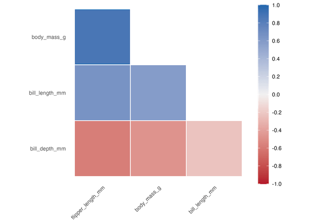
Lower Triangular Correlation heatmap with autoplot()

We can get lower triangular correlation heatmap using triangular=”lower” as argument to autoplot() function. In this example below we have also rearranged the correlation dataframe by its strength.

penguins %>% 
  correlate() %>%
  rearrange() %>%
  autoplot(triangular="lower")
ggsave("corrr_autoplot_heatmap_lower.png")

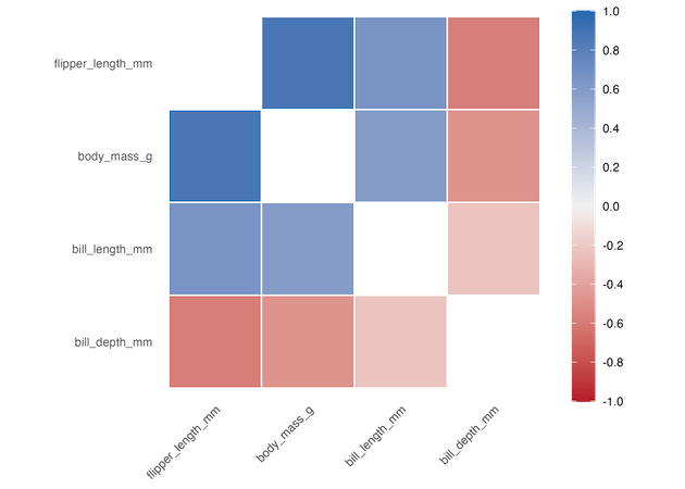
Full Symmetric Correlation heatmap with autoplot()

Similarly, we can get a full symmetric correlation heatmap using triangular=”full” as argument to autoplot() function.

penguins %>% 
  correlate() %>%
  rearrange() %>%
  autoplot(triangular="full")
ggsave("corrr_autoplot_heatmap_full.png")

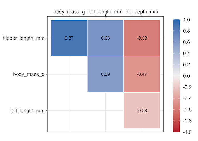
Annotating Correlation heatmap with autoplot()

One of the biggest advantages of using corrr to visualize correlation is that, the resulting object is a ggplot2 object. This gives us freedom to further customize the correlation heatmap. For example, in the example below we have annotated the heatmap by adding the actual correlation value we computed using correlate(). We have added another layer to the plot using geom_text() function in ggplot2.

penguins %>% 
  correlate() %>%
  rearrange() %>%
  autoplot()+
  geom_text(aes(label=round(r, digits=2)), size=4)+
  theme_bw(16)
ggsave("corrr_autoplot_heatmap_annotated_upper.png")